Primer: Critical Batch Size — the Optimizer Ceiling
Primer: Critical Batch Size — the Optimizer Ceiling
Section titled “Primer: Critical Batch Size — the Optimizer Ceiling”The hardware roofline sets a floor on per-chip batch (see pod-scale training §2); this primer is the ceiling — the training-dynamics side of “how big should the batch be.” Five paragraphs, each one load-bearing.
1. Why there is a ceiling at all. A minibatch gradient is a noisy estimate of the true gradient; batch size B averages B samples of that noise, shrinking its variance by 1/B. While noise dominates the update, doubling B nearly halves the number of steps to reach a given loss — batch size is free parallelism, converting wall-clock into width. But once the noise is small relative to the true gradient, further averaging polishes a signal that was already clean: doubling B buys almost no step reduction, so tokens-to-target-loss inflates and you are spending compute to go the same distance. The crossover between those regimes is the critical batch size B_crit. Below it, big batches are how you use a big machine; above it, they are how you waste one.
Tokens to reach target loss (E) Steps to reach target loss (S) │ │ 4·E_min┤ × S_min·8┤× │ × │ × 2·E_min┤ × │ × "perfect │ × S_min·2┤ × scaling": E_min ┤×──×──×──× ← flat: extra │ × 2×B → S/2 │ batch is free S_min ┤ ×──×──×──× └┬──┬──┬──┬──┬──┬──┬──┬─ B └┬──┬──┬──┬──┬──┬──┬─ B ↑ B_crit (the knee) ↑ B_crit Left: below B_crit, tokens-to-loss is constant — parallelism is free. Right: above B_crit, steps stop shrinking — wall-clock stops improving. Same knee, seen from the compute side and the time side.2. The canonical framework: gradient noise scale. McCandlish, Kaplan, Amodei et al., “An Empirical Model of Large-Batch Training” (2018), is the paper that gave this a number: the noise scale — per-sample gradient noise variance over squared true-gradient norm — and the empirical claim that . Its central prediction is that the two curves above are one hyperbola: steps S and examples E to reach a given loss trade off as
with B_crit sitting at the elbow — the paper’s Figure 1 draws the consequence for planning: pick a point on the frontier by deadline and budget, not by habit. Canonical is not definitive: the noise scale is a heuristic (it ignores curvature anisotropy, interacts with the LR schedule, and its Adam variant is rougher than the SGD theory), and it can be off by small multiples — but it matched measured Pareto fronts across supervised, RL, and generative tasks, its curve shape was independently confirmed at scale by Shallue et al., “Measuring the Effects of Data Parallelism” (2018), and it remains the shared vocabulary of every batch-size conversation since.
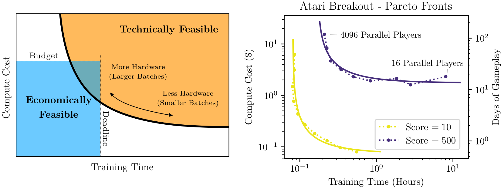
3. B_crit is not a constant — it grows during training. As loss falls, the true gradient shrinks faster than its per-sample noise, so rises — often by 10–100× over a pretraining run. This single fact explains batch warmup: early training might only support a few million tokens usefully (a 37M-token batch there wastes most of its compute), while late training supports tens of millions — DeepSeek-V3 ramping its batch to ~60M tokens is this curve made into a schedule. The important modern refinement is Zhang et al., “How Does Critical Batch Size Scale in Pre-training?” (2024): B_crit scales primarily with data consumed / loss progress, not with model size — a bigger model does not by itself license a bigger batch; being further along the loss curve does. Practical consequence: batch schedules should key off training progress, and a batch chosen for the end of the run is the maximum of the schedule, not its constant.
Batch (tokens, log scale) │ B_crit(t) ~ noise scale: 60M ─┤ ╭────── rises as ‖g‖² falls │ ╭───────╯ ┌──────── ← actual batch schedule 30M ─┤ ╭─────╯ ┌────┘ (staircase chasing │ ╭───╯ ┌───┘ B_crit from below) 10M ─┤ ╭───╯ ┌───┘ │ ╭──╯ ┌──────┘ waste zone: batch > B_crit(t) 3M ─┤─╯──────┘ (early big batch = polishing clean grads) └────────┬──────────┬──────────┬──────── training progress early mid late (tokens seen)4. How you actually measure it. Three instruments, in increasing cost. (a) Live noise-scale estimation, nearly free: with data parallelism you already hold per-replica gradients; McCandlish et al.’s Appendix A estimator needs only the gradient norms at two effective batch sizes — the per-replica norm ‖G_small‖² and the all-reduced norm ‖G_big‖² give unbiased estimates of both tr(Σ) and ‖g‖², so the same per-slice grad-norm telemetry a large run keeps for silent-data-corruption detection doubles as a B_crit sensor. (b) Batch-size sweeps at ablation scale: train the small proxy model at several batch sizes with per-batch-tuned LR and plot tokens-to-target-loss vs B (the left curve above); the knee is your number, and per-B LR tuning is non-negotiable — an untuned sweep measures your LR schedule, not the noise scale, and the point where the naive linear-LR-scaling rule stops working is itself corroborating evidence you’ve reached B_crit. (c) Literature anchors (published frontier schedules) bound plausibility but never substitute for (a) and (b) on your own model/data — B_crit is a property of your loss landscape and data distribution.
5. Why a systems interview cares. B_crit is the term that closes the sizing loop: the ICI roofline gives a per-chip token floor (≈2,550/M_X on v5p), B_crit gives the global token ceiling, and ceiling ÷ floor caps how many chips can ever be productive on the run:
per-chip tokens = global batch / useful DP extent ───────────────────────────────────────────────────────────── floor: 2,550/M_X ≈ 1,275 ▓▓▓▓│ usable window │ (comms-bound below) ───┤ ├─── ceiling: │ 17,920 chips @ 2,048 ✓ │ B_crit(t) │ │ ≈ 60M late max productive fleet ≈ ceiling / floor ≈ 60M / 1,275 ≈ 47K chips ───────────────────────────────────────────────────────────── …and the window is time-dependent: early in the run B_crit(t) is small, the window narrows, and the schedule (or a sub-mesh) must keep per-chip batch inside it.At a ~60M late-run ceiling and ~1,275-token floor, that’s ~47K chips; scaling past it, no parallelism layout can save you, because the batch that keeps chips compute-bound is a batch the optimizer can no longer use. That is the staff-level answer to “you get 4× the chips overnight”: the constraint that breaks first is not topology or DCN, it is that global batch outruns B_crit — so you shrink per-pod batch back toward the roofline floor and spend the extra chips somewhere else (a second run, faster ablations) once the floor is reached. Batch size is where optimizer statistics and torus topology meet; knowing which side binds, and when during the run it flips, is the whole game.
Sources: McCandlish et al. 2018 (gradient noise scale, the S–E hyperbola, and Figure 1 reproduced above — the framework); Shallue et al. 2018 (empirical scaling curves across workloads); Zhang et al. 2024 (B_crit scales with data, not model size); DeepSeek-V3 report (production batch-ramp schedule); JAX scaling book (the hardware-floor side of the same trade).